A Quick Introduction to P-values

This article can be used both as a stand-alone reference or as Part 2 of our series on making a p-value calculator web app. Please see Part 1 for an overview of this project.

Introduction

In this series, we develop a webapp for calculating a "p-value," a useful value that descibes the probability of a set of observations. In the webapp, the user is prompted to input a t-statistic and a corresponding p-value is returned. We could have made a simple addition calculator, but I thought it better to create a tool that is a bit less ubiquitous, and therefore, useful. The concept of a p-value is not too complicated. We will illustrated it with an example.

An Instructive Example

Suppose that we have a random sample of people. The average height of individuals in this sample of 64 inches. We might be curious as to the probability that the respective populations from which this groups was sampled actually has an average height of 63 inches. In other words, we are interested in the probability that drawing the mean height of 64 inches was "just by chance," as opposed to the mean height in the population really not being 62 inches.

Of course, the practical significance of the 1-inch difference is relative: it depends on the internal "spread" of heights within the group. For instance, if the "average spread" of heights within the group is only 0.5 inches (e.g., 64.5, 63.5, 64.0, 64.0. 63.0, 65.0), then the 1-inch gap is pretty large. Conversely, if if the "average spread" of heights within the group is 5 inches (e.g., 54, 59, 64, 64. 69, 74), then the 1-inch gap is pretty small. For reasons that are not so important for our present purposes, we don't actually consider the "average spread", but rather a descriptive statistic called the "standard deviation." For our example, let's say the standard deviation is 1 inch. It also depends on how many individuals are in our group: the more individuals there are, the more confident we can be that the mean height in the population is close to 64 inches ("the law of large numbers"). For our example, let's say that the sample size is 9.

The one-sample t-test forumula simulatenously accounts these three factors: 1) the 1-inch difference in heights, 2) the 1-inch standard deviation in heights within our group, and 3) the sample size of 9:

... where $\overline{x}$$\bar{x}$ is the sample average of 64, $\mu$$\mu$ is the population average of 63, $s$$s$ is the sample standard deviation of 1, and $n$$n$ is the sample size of 16. Therefore, $t$$t$ is $(64-63)/(1/3)$$(64-63)/(1/3)$ ...or $3$$3$​.

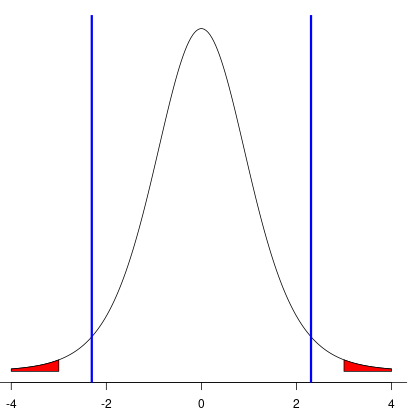
Notice that the shaded red area under the t-distribution in the diagram starts at 3 and -3, corresponding the to the t-statistic that we just calculated. It turns out that this red area constiutes 1.7% of the area under the curve (the area to the left and right of the blue verticle lines represents 5% of the area under the curve) This means that if the mean height of the population from which our sample was drawn really were 63, we would only expect to see results at least as extreme as ours (i.e., with a sample mean of 64 or above, or 62 or below) 1.7% of the time, given we found ourselves in this exact situaion an infinite number of times. Is this a lot or a little? It depends on the context, but under many circumstances we might assume that our sample was drawn from a population that did not have a mean height of 63. In statistics, this assumption is refered to as "rejecting the null hypothesis that $\mu =63$$\mu = 63$". This value of 1.7%, or 0.017, is refered to as a "p-value."

Conclusion

Hopefully, this sheds some light on the concept of t-statistics and p-values. However, please keep in mind that for the purposes of this tutorial series, understanding these concepts is not strictly necessary. Of course, it's nice to be able to appreciate the practical utility of the tool that we are building.